
Fiber photometry#
Fiber photometry is an in-vivo optical recording technique for measuring the bulk activity of a genetically defined neuron population in a freely moving animal. The technique is widely used in systems neuroscience to characterize brain-behaviour relationships at the level of defined circuits and cell types (Simpson et al. 2024).
The signal it produces is a single fluorescence trace, generated by a genetically encoded indicator expressed in the target cells. Indicators exist for many molecules (calcium, individual neurotransmitters, intracellular signaling messengers); this explainer uses GCaMP, a calcium sensor, as the running example because it is the most widely used and the one whose development drove photometry’s adoption. GCaMP turns intracellular calcium into emitted light, and intracellular calcium rises when neurons fire, so the fluorescence trace serves as a proxy for the labeled population’s spiking activity.
Three qualities of fiber photometry drive its adoption:
Cell-type specificity through genetic targeting. The indicator is expressed only in neurons defined by viral promoter or Cre-driver line, so the recording is restricted to a chosen population rather than every neuron near the fiber.
Access to deep brain structures. The implanted fiber reaches subcortical regions that surface optical methods (two-photon imaging, mini-scopes) cannot.
Naturalistic behaviour. No head-fixation and no microscope rigging during the session; the fiber implant is mechanically robust enough for long recording sessions in freely moving animals, across days, weeks, or months.
Experimental setup#
Each of those qualities is grounded in a specific part of the apparatus. The schematic below traces the experiment end to end.
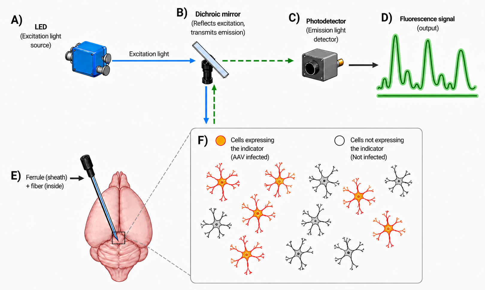
The indicator’s genetic construct is delivered by an adeno-associated virus (AAV) injection into the target brain region (a separate surgery, not depicted). The construct is gated by a viral promoter, often combined with a Cre-driver line in transgenic animals, and that promoter-plus-Cre combination is what gives photometry its cell-type specificity: only neurons that match the genetic targeting begin expressing the indicator (the orange cells in inset F). Cells that the virus does not reach, or that do not match the targeting, remain unlabeled (grey) and contribute nothing to the recording. This is the experimental knob the experimenter has over which cells they end up reading from.
The optical fiber implant (E) is placed into the same region in a separate surgery. The implant is a two-part unit: an outer ferrule (typically a small ceramic sleeve) that anchors mechanically to the skull with dental cement, and an inner light-carrying fiber (~200-400 µm core diameter for typical photometry experiments) bonded inside the ferrule. The ferrule provides a standardized optical connector for a patch cable that links the implant to the bench-top optics, so the apparatus can be detached between sessions and reattached repeatably across weeks. The fiber descends to wherever in the brain a needle can reach, so subcortical regions inaccessible to surface-only methods become recordable. Once implanted, the fiber carries light in both directions simultaneously: excitation light going down to the tissue, emitted fluorescence coming back up.
An important feature of fiber photometry, and of fluorescence microscopy more generally, is how a dichroic mirror (B) lets two light signals share the same optical path. On the bench, an LED (A) delivers excitation light at the wavelength that drives the indicator (~470 nm, blue, for GCaMP). That light hits the dichroic, which is a wavelength-selective beam splitter: it reflects light below a chosen cut-on wavelength and transmits light above it. With the cut-on placed between GCaMP’s excitation peak (~470 nm) and emission peak (~525 nm), the dichroic enables two distinct light paths through one fiber:
Excitation: blue path going down. Blue light from the LED arrives at the dichroic at 45°; because it sits below the cut-on, the dichroic reflects it at 90° downward into the optical fiber and into the tissue.
Emission: green path coming up. Green fluorescence emitted by the indicator travels back up the same fiber to the dichroic; because it sits above the cut-on, the dichroic transmits it straight through to the photodetector.
Without a dichroic, the geometry would require either two separate fibers (one for delivery, one for collection) or a generic 50/50 beam splitter that loses half the light in each direction. With the dichroic, one component handles both directions at near-perfect efficiency, so a single thin fiber is enough. That single-fiber geometry is what keeps the implant minimally invasive: only one insertion surgery is required, the assembly stays small and light enough for the animal to wear across long sessions, and the recording is compatible with freely-moving behaviour.
The nature of the fluorescence signal#
The photodetector (C) (typically a femtowatt photodiode or a photomultiplier tube, chosen for high gain at very low light levels) receives the emission photons that came back through the fiber and the dichroic, and converts them into a voltage trace. That voltage trace is the fluorescence signal (D): a single number per timepoint.
Going from the photodetector back to the tissue, that single voltage emerges from light integrated across a whole population of cells inside the illuminated volume, and that population is heterogeneous. Some cells are responding to the current behavioural event, others are not; some are excited by it, others may be inhibited; cells closer to the fiber tip contribute more emission than cells farther away; each cell’s response unfolds on its own timescale, set by its calcium dynamics and the indicator’s binding kinetics. The fluorescence trace is what you get when light from this population, varying in activity, position, and timing, lands on a single sensor at each instant. What you record, in short, is a weighted optical sum over a sampling volume below the fiber tip. Three properties of the trace follow from that view: aggregation across cells (which collapses the variation in activity), spatial extent (set by the cells’ positions in the volume), and temporal shape (set by each cell’s kinetics).
Aggregation across cells. The signal at any timepoint is the algebraic sum of emission from every labeled cell in the volume. Cells that are firing contribute more (calcium up, GCaMP brighter); quieter cells contribute less; the photodetector reads out the sum as a single voltage. Figure 2 makes the construction concrete: a labeled population, each cell with its own response trace heterogeneous in timing, amplitude, and shape, and the bulk sum overlaid in bold. The sum is the signal.

Spatial extent. The signal is sampled from a cone of tissue under the fiber tip, the volume the fiber both illuminates with excitation light and collects emission from. Its size is set by the fiber’s core diameter and numerical aperture, modulated by scattering and absorption in brain tissue: most of the fluorescence comes from cells within a few hundred micrometers of the tip, with contributions tapering off rather than ending sharply. Within that volume, contribution to the sum is weighted by collection efficiency rather than mapped to position; a cell at the tip and a cell 300 µm away both feed the same scalar.
Temporal shape. The trace is a low-pass-filtered version of population spiking. Several sources of blur stack together: an action potential triggers calcium influx that takes ~10 ms to peak, the indicator binds and unbinds calcium with its own kinetics, and intracellular calcium buffers compete with the indicator for free calcium and slow both rise and decay. GCaMP variants explicitly trade speed for brightness (slower variants such as GCaMP6s give a stronger signal at the cost of a longer decay; faster variants such as jGCaMP8 reverse the trade), and the figure in the next section places each variant on the time axis.
These three properties together explain a practical reading note: the same bulk peak can come from very different population states, since the algebraic sum is not invertible. Broad labeling that captures cells with opposite-polarity responses can produce partial or full cancellation; the canonical case is striatum, where D1 and D2 medium spiny neurons respond oppositely to reward (Cui et al. 2013), which is why that population is recorded with subtype-selective Cre lines rather than a pan-neuronal marker. Within a Cre-targeted population, the typical consequence is amplitude attenuation rather than full cancellation; the bulk readout cannot distinguish a small response from a partially attenuated one.
Photometry and other experimental methods#
Photometry occupies a specific corner of the recording-methods space, defined by four niche properties: cell-type-specific recording, access to deep brain regions, compatibility with freely-moving animals, and recording sessions that last weeks, all at comparatively modest hardware cost and surgical complexity. The price is cellular resolution and millisecond timing.
Among those four properties, longitudinal stability is photometry-specific among nearby techniques: a ferrule-mounted fiber implant survives weeks to months, while miniscope and cranial-window setups face progressive scarring, fluorescence dropout, or physical wear that often caps stable recording at days to weeks. Each peer technique below restores one of the two precisions but loses one of the four niche properties; the comparison shows which axis you would give up by reaching for a different tool.
The figure below maps photometry against three peer techniques on time and space, the two precision axes. The four niche properties are not on the figure but matter just as much for tool selection.

The shaded gray range (~50 ms to ~30 s) marks the behaviourally relevant timescale, from whisks and licks at the fast end through operant trials and sustained cues at the slow end.
Two-photon imaging answers which cells within the population responded, at the cost of head-fixation and a cranial window. Picking two-photon over photometry trades freely-moving compatibility for cellular detail.
Microendoscopy / miniscope answers which cells responded in a freely-moving animal, at the cost of a more invasive GRIN lens, a bulkier headstage, and shorter session-to-session stability. Picking miniscope trades longitudinal stability for cellular detail.
Electrophysiology, particularly Neuropixels, answers when spikes occurred and which units fired, at the cost of needing extra steps (opto-tagging, etc.) to identify which units belong to which genetically defined cell type. Picking Neuropixels trades genetic cell-type identity for spike-level precision.
fMRI answers how activity is distributed across the whole brain, at the cost of an indirect (BOLD) and slow (second-scale) signal with no cell-type targeting. It serves more as an outer bound than a direct competitor.
Other techniques fill the rest of the landscape, including voltage imaging (sub-millisecond optical analogue of patch-clamp), wide-field calcium imaging (cortical-area through a cranial window), and the bulk-electrical methods (LFP, EEG, MEG, in a different signal domain). Each is the right tool for specific questions but does not illuminate photometry’s niche axes more sharply than the four comparators above.
Photometry is the right tool when the question is about a genetically defined population’s activity over seconds, in an animal that is moving, across a recording session that lasts weeks. It is the wrong tool when the question is about single cells, fast spike timing, or finer spatial structure, where the comparators above are the answer. Many cells, one trace: that is photometry’s central idea.